Abstract
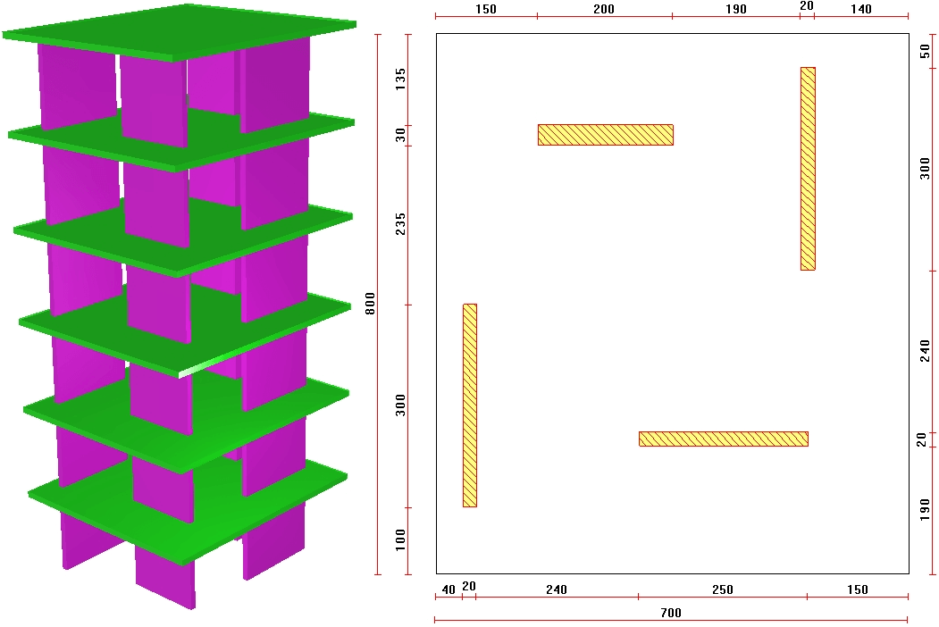
The aim of the seismic analysis is to calculate the reaction of the model to earthquakes. This example describes the method to analyze the structure using Modal Analysis. Modal Analysis is the accepted method and is recommended by most design codes. The reaction of the model for each mode shape is calculated according to the response spectrum given by the seismic code. Because the aim of this example is to describe the method to perform Modal Analysis, we will use a simple six-story structure, with a story height of 3 meters. The seismic load carrying system consists of four shear walls.
Geometry Definition
We will define the model geometry and part of the loads using the AutoSTRAP program.
The DXF file can be downloaded from EX4.DXF
AutoSTRAP
- click the AutoSTRAP
 icon on the desktop or from STRAP’s models tab click Utilities > AutoSTRAP.
- click the “New” icon
 or click File > New-import DXF file.
 - select the DXF file that you downloaded and click open.
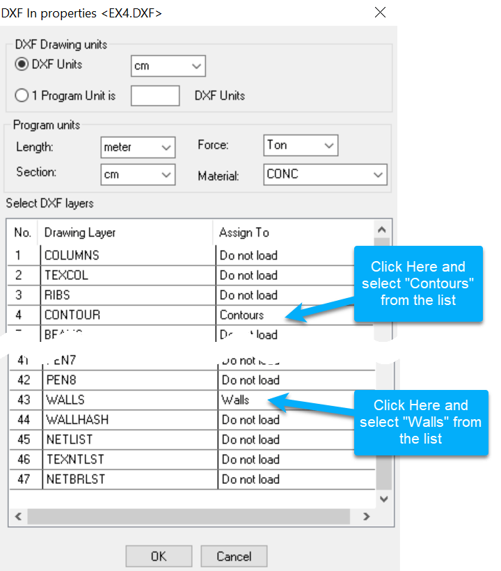
- the program displays the following menu. The lines representing the contours are found in Layer #4 and the lines forming the walls are in Layer #43 and these layers must be identified and assigned:
- the elements identified by the program are displayed on the screen. To display the slab element grid, click on the
 icon.
icon. - click on
 in the side menu and Add Level at the bottom of the dialog box:
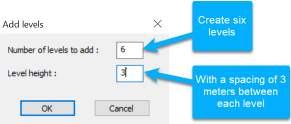
- The program adds the list of levels to the Dialog box. click End to continue.
- Click
 in the lower side menu, then select
  in the upper side menu.
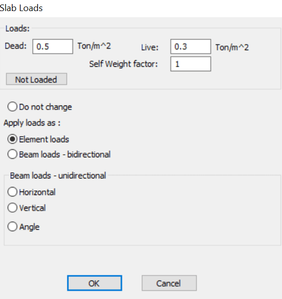
 - Click Select all spaces and define the loads:
- Create the STRAP model: click
 in the bottom side menu.
 - Click
 in the top side menu and check
  Create rigid links in plane. This option creates infinite rigidity in the plane of the floor slab.
 - Click
 in the top side menu
STRAP
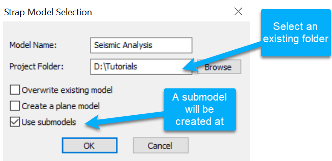
Run STRAP and open the created model Seismic Analysis.
- click
 in the icon bar to display an isometric view.
 - select the submodel to display from the list in the side menu:

- click
 in the icon bar to display the walls.
 - define “dummy beams” on the slab perimeter (for applying line loads to the slab): click
 in the lower side menu, then click
  in the upper side menu.
 - Set the following two parameters:
- Prop. = 0 in the bottom dialog box (indicates that the beams are ‘dummy’).
 Chain with the previous beam in the options at the top of the side menu.
- Select the four corner nodes in sequence, then select the first node again to end the beam definition.
- display the Main model:

Loads Definition
Add the walls self-weight and the masonry line loads along the slab perimeter (the slab self-weight was defined as part of the slab dead load):
- click the
 tab.
tab. - select
 in the side menu, select the “Dead” load case and click
  .
. - select
 in the lower side menu and select
  in the upper side menu.
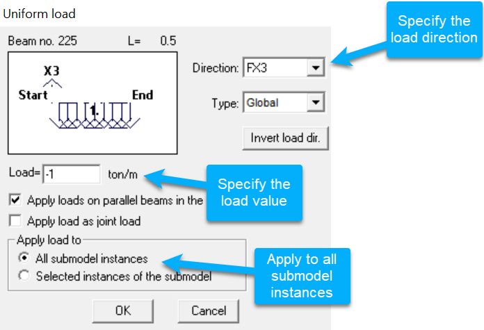
 - click on
 , select the local x3 direction and define a factor = -1.0.
 - click on Select all walls; the load is applied to all the walls in the main model.
- select the first instance of the submodel:

- select
 in the lower side menu and select
  in the upper side menu.
 - click on
 , then Select all beams and define the loads:
- return to the Main model:

- click

- click
 to solve the model for static loadsץ
Modal Analysis
- click the
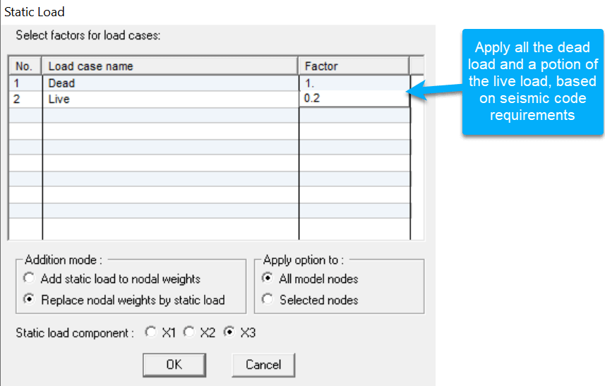
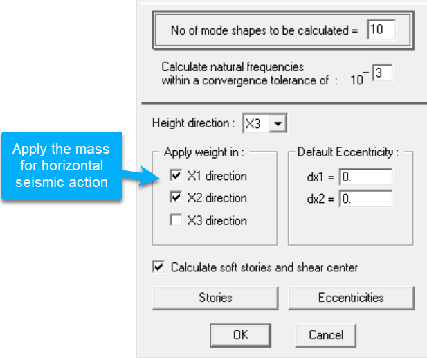
 tab. The masses are defined from the static loads.
 - select the
 option:
- select
 in the side menu:
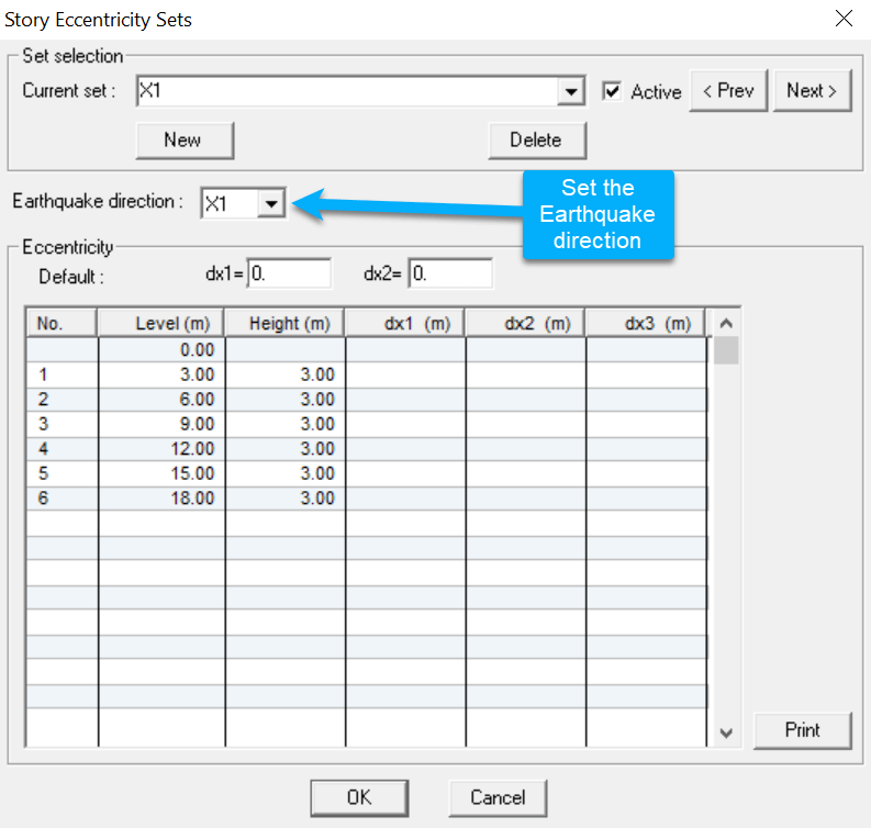
- click the
 button to define an earthquake in the X1 direction.
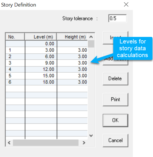
- click the
 to verify the levels for Story data calculations.
- click
 to calculate the mode shapes. After the modal analysis is solved, you will get into the
  tab.
tab. - display the results graphically: select a mode shape and then click Start Animation / End Animation at the bottom of the screen to start/stop animation; repeat for other mode shapes.
Seismic Analysis
- Select the method for combining the modes: select Seismic analysis in the menu bar and Method for combining modes in the pulldown menu:
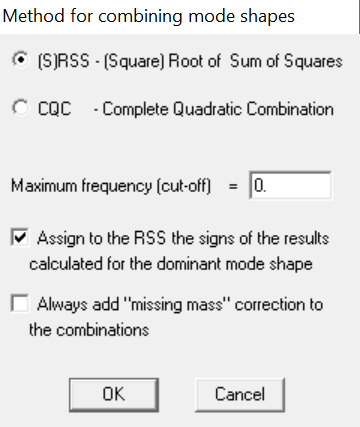
SRSS: square root of the sum of squares. The estimated response R (force, displacement, etc) at a specified coordinate is expressed as:
![]()
where Ri is the corresponding maximum response of the ith mode at the coordinate.
CQC: complete quadratic combination. The estimated response is expressed as:
![]()
where ρ = the cross-modal damping coefficient.
Note:
* When some of the modes are closely spaced, the SRSS method may grossly underestimate or overestimate the maximum response. Large errors have been found in particular in space models in which the torsional effects are significant. The term “closely spaced” may be arbitrarily defined as the case where the difference between two natural frequencies is less than 10% of the smaller frequency.
* The CQC method is a more precise method of combining the maximum values of the modal response.
* The two methods are identical for undamped models (x = 0).
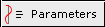
The seismic analysis for this example is done according to the ASCE/SEI 7-16 Code; you may select other Codes, e.g., Eurocode 8, NBC-Canada, etc.
- select
 in the side menu:
- Specify the direction that the earthquake is applied. Select one of the global directions or define a vector as a combination of the three global directions. All mode shapes are used no matter in which direction the earthquake is applied. However, the modes which have deflections in the applied direction will dominate.
- Specify the soil type as per Table 20.3.1.
- Define the Importance factor as per Table 11.5.1.
- Define the “Response modification coefficient” as per Table 12.2-1.
- Specify a value of TL, calculated according to Section 11.4.5 and the Figures in Chapter 22.
- Specify the mapped maximum considered earthquake spectral response acceleration at short periods (Ss) and at 1s (S1) as detailed in Section 11.4 and the Maps in Section 20.
- Referring to Section 12.9.4, when the base shear calculated from the modal shape analysis is different than the base shear calculated according to the Equivalent lateral force procedure of Section 12.8, all corresponding responses, including moments and forces, are adjusted accordingly.
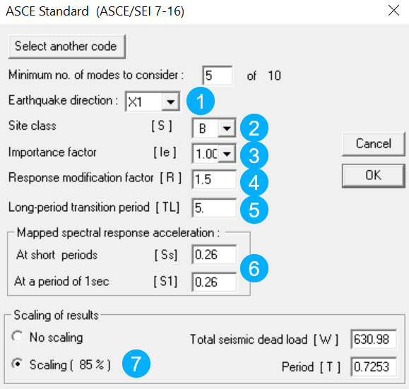
- to display the modal results, click
 and select
  .
.
- period (seconds)
- Participation factor: a factor reflecting the relative influence of the mode shape. The sum should be greater than 90%.
- the sum of external forces in all global directions.
- the root of the sum of the squares of the horizontal forces.
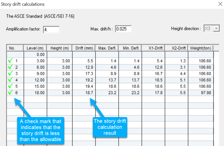
- click
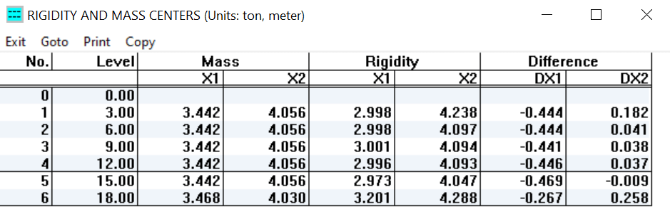
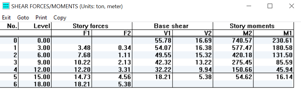
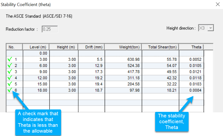
 to display the story data results at each level:
 - Drift Calculations
- Stiffness and mass center
- Story shear forces and moments
- Stability coefficient (Theta)
- Weak story

- Soft story
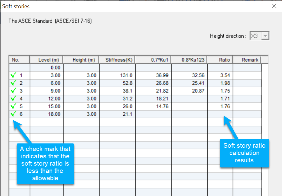
- click
 in the side menu to Create static load cases from the modal results and append them to the regular load cases:
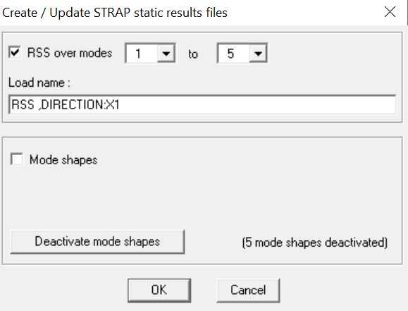
The program creates a fictitious load case representing an earthquake acting in the X1 direction, created by combining the mode shapes according to the code. The step should be repeated for the X2 direction, but the following steps assume that only this one case was created. In addition, we have not considered the minimum eccentricity required by the code.
Results
- click the
 tab.
tab. - display only the main model: select Display, Submodel instances and remove all; click OK..
- click
 and select the options in the following menu:
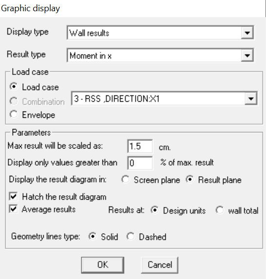
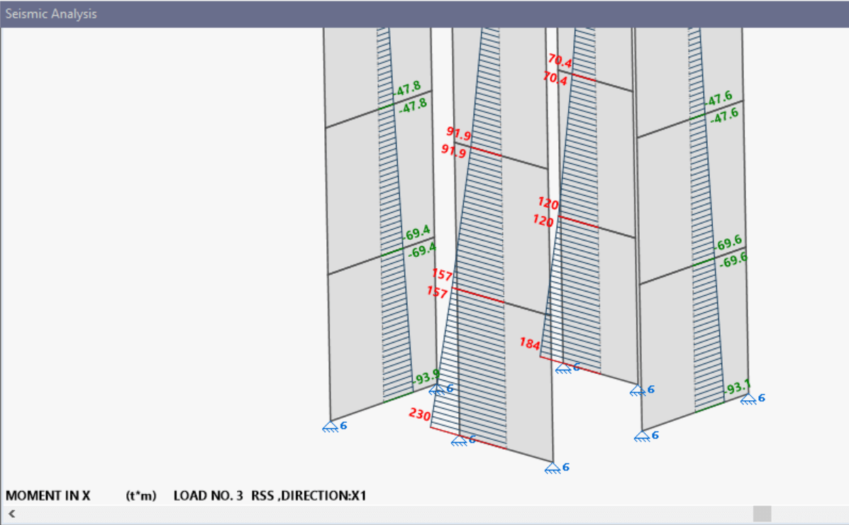
The program displays Moment in the X direction for each wall design unit.
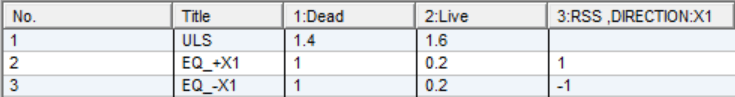
- create combinations: select
 in the lower side menu,
  in the upper side menu and create the following combinations: